Image Classifiers with Tensorflow 2.0
This project explores Tensorflow 2.0 using Keras to build image classifiers in two different ways.
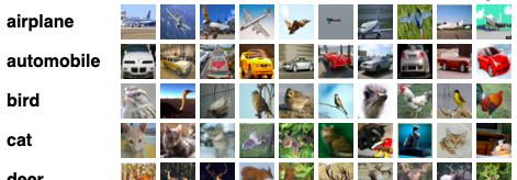
 Sample images from: CIFAR-10 dataset
Recently when Tensorflow 2.0 was released, a number of changes occurred including the integration of Keras as the official highlevel API for Tensorflow. Keras allows models to be defined in three ways: sequentially, functionally, and through subclassing. This project will build the three image classifiers using these two methods: sequential, and functional. Thanks to pyimagesearch for the guide on how to do this.
The first model will be a simple shallow CNN. The second model will be a simplified version of the GoogleNet (a much more complex model that justifies the use of the functional model for defining models):
@misc{szegedy2014going,
title={Going Deeper with Convolutions},
author={Christian Szegedy and Wei Liu and Yangqing Jia and Pierre Sermanet and Scott Reed and Dragomir Anguelov and Dumitru Erhan and Vincent Vanhoucke and Andrew Rabinovich},
year={2014},
eprint={1409.4842},
archivePrefix={arXiv},
primaryClass={cs.CV}
}
They will be trained and tested against the CIFAR 10 database: Learning Multiple Layers of Features from Tiny Images, Alex Krizhevsky, 2009.
I will also explore how to export data to Tensorboard using Tensorflow 2.0 which has moved away from using sessions.
Lastly, I will use an AWS EC2 instance. Note about this is that AWS performed the first fitting reasonably faster than my CPU (2-3x), but it performed the second fitting on the MiniGoogleNet much faster (a couple minutes per epoch vs a couple hours per epoch).
Note 2: I originally tried using tfds to load this data and use tensorflow dataset objects to do this project, however tensorflow datasets don’t play nicely with keras preprocessing modules. Datasets are lazy loaded so all preprocessing on datasets must be done through mapping functions and not on the data directly. These mapping functions must act on tensors natively. However Keras preprocessing modules are unable to be used as mapping functions because they only work on numpy arrays.
Import libraries and data
import tensorflow as tf
import tensorflow.keras as tk
%load_ext tensorboard

#import tensorflow_datasets as tfds
from tensorflow.keras.datasets import cifar10
import numpy as np
import datetime
from sklearn.metrics import classification_report
import tensorflow.keras.preprocessing.image as image
from tensorflow.keras.optimizers import SGD
from sklearn.preprocessing import LabelBinarizer
#data, info = tfds.load(name='cifar10', with_info=True)
(trainX, trainY), (testX, testY) = cifar10.load_data()
Downloading data from https://www.cs.toronto.edu/~kriz/cifar-10-python.tar.gz
170500096/170498071 [==============================] - 8s 0us/step
#info
Prep data
lb = LabelBinarizer()
trainX, testX = trainX.astype('float32')/255.0, testX.astype('float')/255.0
trainY, testY = lb.fit_transform(trainY), lb.fit_transform(testY)
#def map_function(data):
#    x = tf.cast(data['image'], 'float')/255.
    #x = image.random_rotation(x, 18)
    #x = image.random_zoom(x, 0.15)
    #x = image.random_shift(x, wrg =0.2, hrg=0.2)
    #x = image.random_shear(x, 0.15)
    #x = image.random_left_right(x)
#    data['image'] = x
#    data['label'] = tf.one_hot(data['label'], depth=info.features['label'].num_classes)
#    return data
#train, test = data['train'].map(map_function), data['test'].map(map_function)
#for sample in train.batch(1).take(1):
#    print(sample)
#classes = {
#    'names' : info.features['label'].names,
#    'num_classes' : info.features['label'].num_classes
#}
#classes['names']
Shallownet using Keras sequential
def shallownet_sequential(height, width, depth, classes):
    model = tk.models.Sequential()
    input_shape = (height, width, depth)

    # add layers
    model.add(tk.layers.Conv2D(32, (3,3), padding='same', input_shape=input_shape))
    model.add(tk.layers.Activation('relu'))

    model.add(tk.layers.Flatten())
    model.add(tk.layers.Dense(classes))
    model.add(tk.layers.Activation('softmax'))

    return model
Training the Shallownet
aug = image.ImageDataGenerator(
    rotation_range=18,
    zoom_range=0.15,
    width_shift_range=0.2,
    height_shift_range=0.2,
    shear_range=0.15,
    horizontal_flip=True,
    fill_mode='nearest'
)
# hyperparameters
init_lr = 1e-2
batch_size = 128
num_epochs = 30

# create model, create optimizer, compile model
model = shallownet_sequential(32, 32, 3, testY.shape[1])
opt = SGD(lr=init_lr, momentum=0.9, decay=init_lr/num_epochs)
model.compile(loss='categorical_crossentropy', optimizer=opt, metrics=['accuracy'])

# create tensorboard callback
log_dir = 'logs/fit/' + datetime.datetime.now().strftime('%Y%m%d-%H%M%S')
tb_callback = tk.callbacks.TensorBoard(log_dir=log_dir, histogram_freq=1)

# train model
H = model.fit_generator(
    aug.flow(trainX, trainY, batch_size=batch_size),
    validation_data = (testX, testY),
    steps_per_epoch = int(len(trainX)/batch_size),
    epochs=num_epochs,
    verbose=1,
    callbacks=[tb_callback]
)
Epoch 1/30
  1/390 [..............................] - ETA: 7:09:04 - loss: 2.3224 - accuracy: 0.0859WARNING:tensorflow:Method (on_train_batch_end) is slow compared to the batch update (0.714192). Check your callbacks.
390/390 [==============================] - 101s 258ms/step - loss: 1.9210 - accuracy: 0.3139 - val_loss: 1.7376 - val_accuracy: 0.3680
Epoch 2/30
390/390 [==============================] - 36s 91ms/step - loss: 1.7396 - accuracy: 0.3780 - val_loss: 1.5518 - val_accuracy: 0.4550
Epoch 3/30
390/390 [==============================] - 36s 92ms/step - loss: 1.6406 - accuracy: 0.4130 - val_loss: 1.4179 - val_accuracy: 0.4986
Epoch 4/30
390/390 [==============================] - 35s 91ms/step - loss: 1.5954 - accuracy: 0.4282 - val_loss: 1.3994 - val_accuracy: 0.5025
Epoch 5/30
390/390 [==============================] - 35s 90ms/step - loss: 1.5775 - accuracy: 0.4329 - val_loss: 1.4838 - val_accuracy: 0.4801
Epoch 6/30
390/390 [==============================] - 36s 91ms/step - loss: 1.5477 - accuracy: 0.4469 - val_loss: 1.3632 - val_accuracy: 0.5154
Epoch 7/30
390/390 [==============================] - 35s 90ms/step - loss: 1.5370 - accuracy: 0.4533 - val_loss: 1.4107 - val_accuracy: 0.5068
Epoch 8/30
390/390 [==============================] - 36s 92ms/step - loss: 1.5116 - accuracy: 0.4600 - val_loss: 1.3832 - val_accuracy: 0.5204
Epoch 9/30
390/390 [==============================] - 35s 90ms/step - loss: 1.5035 - accuracy: 0.4643 - val_loss: 1.3619 - val_accuracy: 0.5155
Epoch 10/30
390/390 [==============================] - 35s 90ms/step - loss: 1.4933 - accuracy: 0.4679 - val_loss: 1.3430 - val_accuracy: 0.5338
Epoch 11/30
390/390 [==============================] - 35s 90ms/step - loss: 1.4850 - accuracy: 0.4701 - val_loss: 1.3995 - val_accuracy: 0.5163
Epoch 12/30
390/390 [==============================] - 35s 89ms/step - loss: 1.4774 - accuracy: 0.4744 - val_loss: 1.3298 - val_accuracy: 0.5312
Epoch 13/30
390/390 [==============================] - 35s 90ms/step - loss: 1.4709 - accuracy: 0.4741 - val_loss: 1.3276 - val_accuracy: 0.5356
Epoch 14/30
390/390 [==============================] - 35s 90ms/step - loss: 1.4633 - accuracy: 0.4778 - val_loss: 1.3807 - val_accuracy: 0.5291
Epoch 15/30
390/390 [==============================] - 35s 89ms/step - loss: 1.4577 - accuracy: 0.4830 - val_loss: 1.3219 - val_accuracy: 0.5386
Epoch 16/30
390/390 [==============================] - 35s 90ms/step - loss: 1.4479 - accuracy: 0.4854 - val_loss: 1.3449 - val_accuracy: 0.5258
Epoch 17/30
390/390 [==============================] - 35s 89ms/step - loss: 1.4377 - accuracy: 0.4877 - val_loss: 1.2829 - val_accuracy: 0.5537
Epoch 18/30
390/390 [==============================] - 35s 90ms/step - loss: 1.4375 - accuracy: 0.4906 - val_loss: 1.3120 - val_accuracy: 0.5479
Epoch 19/30
390/390 [==============================] - 35s 89ms/step - loss: 1.4266 - accuracy: 0.4917 - val_loss: 1.3089 - val_accuracy: 0.5449
Epoch 20/30
390/390 [==============================] - 35s 89ms/step - loss: 1.4248 - accuracy: 0.4942 - val_loss: 1.2675 - val_accuracy: 0.5625
Epoch 21/30
390/390 [==============================] - 35s 89ms/step - loss: 1.4166 - accuracy: 0.4983 - val_loss: 1.2683 - val_accuracy: 0.5687
Epoch 22/30
390/390 [==============================] - 35s 89ms/step - loss: 1.4124 - accuracy: 0.4998 - val_loss: 1.2690 - val_accuracy: 0.5602
Epoch 23/30
390/390 [==============================] - 35s 90ms/step - loss: 1.4094 - accuracy: 0.5004 - val_loss: 1.2674 - val_accuracy: 0.5559
Epoch 24/30
390/390 [==============================] - 34s 88ms/step - loss: 1.4078 - accuracy: 0.5013 - val_loss: 1.2632 - val_accuracy: 0.5646
Epoch 25/30
390/390 [==============================] - 35s 89ms/step - loss: 1.4025 - accuracy: 0.5019 - val_loss: 1.2930 - val_accuracy: 0.5577
Epoch 26/30
390/390 [==============================] - 35s 90ms/step - loss: 1.3987 - accuracy: 0.5035 - val_loss: 1.2789 - val_accuracy: 0.5592
Epoch 27/30
390/390 [==============================] - 35s 89ms/step - loss: 1.3947 - accuracy: 0.5036 - val_loss: 1.2645 - val_accuracy: 0.5695
Epoch 28/30
390/390 [==============================] - 35s 90ms/step - loss: 1.3864 - accuracy: 0.5072 - val_loss: 1.2443 - val_accuracy: 0.5688
Epoch 29/30
390/390 [==============================] - 35s 89ms/step - loss: 1.3872 - accuracy: 0.5097 - val_loss: 1.2682 - val_accuracy: 0.5682
Epoch 30/30
390/390 [==============================] - 35s 90ms/step - loss: 1.3814 - accuracy: 0.5107 - val_loss: 1.2377 - val_accuracy: 0.5735
label_names = ["airplane", "automobile", "bird", "cat", "deer", "dog", "frog", "horse", "ship", "truck"]
predictions = model.predict(testX, batch_size=batch_size)
print(classification_report(testY.argmax(axis=1), predictions.argmax(axis=1), target_names=label_names))
              precision    recall  f1-score   support

    airplane       0.58      0.68      0.62      1000
  automobile       0.54      0.87      0.67      1000
        bird       0.58      0.27      0.37      1000
         cat       0.53      0.24      0.33      1000
        deer       0.60      0.40      0.48      1000
         dog       0.49      0.56      0.52      1000
        frog       0.55      0.82      0.66      1000
       horse       0.56      0.71      0.63      1000
        ship       0.74      0.60      0.66      1000
       truck       0.64      0.60      0.62      1000

    accuracy                           0.57     10000
   macro avg       0.58      0.57      0.55     10000
weighted avg       0.58      0.57      0.55     10000
MiniGoogleNet using Keras functional
# convolution module consists of a convolution layer and batch normalization and a relu activation
def conv_module(x, K, kX, kY, stride, chan_dim, padding='same'):
    x = tk.layers.Conv2D(K, (kX, kY), strides=stride, padding=padding)(x)
    x = tk.layers.BatchNormalization(axis=chan_dim)(x)
    x = tk.layers.Activation('relu')(x)
    return x
# each inception module contains a 1x1 convolution, a 3x3 convolution, and then concatenates those layers
def inception_module(x, numK1x1, numK3x3, chan_dim):
    conv_1x1 = conv_module(x, numK1x1, 1, 1, (1, 1), chan_dim)
    conv_3x3 = conv_module(x, numK3x3, 3, 3, (1, 1), chan_dim)
    x = tk.layers.concatenate([conv_1x1, conv_3x3], axis=chan_dim)
    return x
# each downsampling module contains a convolution and a maxpooling then concatenates them
def downsample_module(x, K, chan_dim):
    conv_3x3 = conv_module(x, K, 3, 3, (2,2), chan_dim, padding='valid')
    pool = tk.layers.MaxPooling2D((3,3), strides=(2,2))(x)
    x = tk.layers.concatenate([conv_3x3, pool], axis=chan_dim)
    return x
def minigooglenet_functional(height, width, depth, classes):
    input_shape = (height, width, depth)
    chan_dim = -1

    #input and first convolution module
    inputs = tk.layers.Input(shape=input_shape)
    x = conv_module(inputs, 96, 3, 3, (1,1), chan_dim)

    #two inception modules before a downsampling
    x = inception_module(x, 32, 32, chan_dim)
    x = inception_module(x, 32, 48, chan_dim)
    x = downsample_module(x, 80, chan_dim)

    #four inception modules before a downsampling
    x = inception_module(x, 112, 48, chan_dim)
    x = inception_module(x, 96, 64, chan_dim)
    x = inception_module(x, 80, 80, chan_dim)
    x = inception_module(x, 48, 96, chan_dim)
    x = downsample_module(x, 96, chan_dim)

    #two more inception modules and then an averaging pool and dropout
    x = inception_module(x, 176, 160, chan_dim)
    x = inception_module(x, 176, 160, chan_dim)
    x = tk.layers.AveragePooling2D((7,7))(x)
    x = tk.layers.Dropout(0.5)(x)

    #lastly flatten and apply softmax
    x = tk.layers.Flatten()(x)
    x = tk.layers.Dense(classes)(x)
    x = tk.layers.Activation('softmax')(x)

    #create model to return
    model = tk.models.Model(inputs, x, name='minigoogle.net')

    return model
Training MiniGoogleNet
# hyperparameters
init_lr = 1e-2
batch_size = 128
num_epochs = 30

# create model, create optimizer, compile model
model_mgn = minigooglenet_functional(32, 32, 3, testY.shape[1])
opt = SGD(lr=init_lr, momentum=0.9, decay=init_lr/num_epochs)
model_mgn.compile(loss='categorical_crossentropy', optimizer=opt, metrics=['accuracy'])

# create tensorboard callback
log_dir = 'logs/fit/' + datetime.datetime.now().strftime('%Y%m%d-%H%M%S')
tb_callback = tk.callbacks.TensorBoard(log_dir=log_dir, histogram_freq=1)

# train model
H_mgn = model_mgn.fit_generator(
    aug.flow(trainX, trainY, batch_size=batch_size),
    validation_data = (testX, testY),
    steps_per_epoch = int(len(trainX)/batch_size),
    epochs=num_epochs,
    verbose=1,
    callbacks=[tb_callback]
)
Epoch 1/30
390/390 [==============================] - 158s 406ms/step - loss: 1.6025 - accuracy: 0.4126 - val_loss: 1.9915 - val_accuracy: 0.3232
Epoch 2/30
390/390 [==============================] - 154s 396ms/step - loss: 1.2244 - accuracy: 0.5624 - val_loss: 1.4986 - val_accuracy: 0.5154
Epoch 3/30
390/390 [==============================] - 154s 395ms/step - loss: 1.0624 - accuracy: 0.6267 - val_loss: 1.1216 - val_accuracy: 0.6200
Epoch 4/30
390/390 [==============================] - 155s 398ms/step - loss: 0.9696 - accuracy: 0.6605 - val_loss: 1.7869 - val_accuracy: 0.4653
Epoch 5/30
390/390 [==============================] - 156s 401ms/step - loss: 0.8873 - accuracy: 0.6902 - val_loss: 0.9987 - val_accuracy: 0.6506
Epoch 6/30
390/390 [==============================] - 157s 402ms/step - loss: 0.8242 - accuracy: 0.7118 - val_loss: 1.1000 - val_accuracy: 0.6531
Epoch 7/30
390/390 [==============================] - 156s 401ms/step - loss: 0.7698 - accuracy: 0.7326 - val_loss: 1.5763 - val_accuracy: 0.5822
Epoch 8/30
390/390 [==============================] - 157s 403ms/step - loss: 0.7323 - accuracy: 0.7466 - val_loss: 1.2515 - val_accuracy: 0.6531
Epoch 9/30
390/390 [==============================] - 156s 400ms/step - loss: 0.6930 - accuracy: 0.7624 - val_loss: 0.8443 - val_accuracy: 0.7198
Epoch 10/30
390/390 [==============================] - 157s 401ms/step - loss: 0.6622 - accuracy: 0.7711 - val_loss: 0.7411 - val_accuracy: 0.7491
Epoch 11/30
390/390 [==============================] - 157s 403ms/step - loss: 0.6368 - accuracy: 0.7804 - val_loss: 0.7518 - val_accuracy: 0.7550
Epoch 12/30
390/390 [==============================] - 158s 404ms/step - loss: 0.6153 - accuracy: 0.7891 - val_loss: 0.7244 - val_accuracy: 0.7617
Epoch 13/30
390/390 [==============================] - 157s 403ms/step - loss: 0.5831 - accuracy: 0.8004 - val_loss: 0.6690 - val_accuracy: 0.7853
Epoch 14/30
390/390 [==============================] - 157s 402ms/step - loss: 0.5668 - accuracy: 0.8056 - val_loss: 0.8492 - val_accuracy: 0.7431
Epoch 15/30
390/390 [==============================] - 157s 402ms/step - loss: 0.5572 - accuracy: 0.8105 - val_loss: 0.6854 - val_accuracy: 0.7910
Epoch 16/30
390/390 [==============================] - 159s 408ms/step - loss: 0.5379 - accuracy: 0.8179 - val_loss: 0.6276 - val_accuracy: 0.8003
Epoch 17/30
390/390 [==============================] - 158s 404ms/step - loss: 0.5119 - accuracy: 0.8247 - val_loss: 0.6931 - val_accuracy: 0.7816
Epoch 18/30
390/390 [==============================] - 156s 400ms/step - loss: 0.5087 - accuracy: 0.8272 - val_loss: 0.7576 - val_accuracy: 0.7635
Epoch 19/30
390/390 [==============================] - 156s 399ms/step - loss: 0.4970 - accuracy: 0.8301 - val_loss: 0.5861 - val_accuracy: 0.8111
Epoch 20/30
390/390 [==============================] - 155s 397ms/step - loss: 0.4879 - accuracy: 0.8321 - val_loss: 0.5968 - val_accuracy: 0.8084
Epoch 21/30
390/390 [==============================] - 155s 398ms/step - loss: 0.4741 - accuracy: 0.8370 - val_loss: 0.4554 - val_accuracy: 0.8470
Epoch 22/30
390/390 [==============================] - 156s 401ms/step - loss: 0.4685 - accuracy: 0.8394 - val_loss: 0.6173 - val_accuracy: 0.8042
Epoch 23/30
390/390 [==============================] - 156s 401ms/step - loss: 0.4616 - accuracy: 0.8407 - val_loss: 0.6431 - val_accuracy: 0.7893
Epoch 24/30
390/390 [==============================] - 155s 398ms/step - loss: 0.4451 - accuracy: 0.8483 - val_loss: 0.5811 - val_accuracy: 0.8091
Epoch 25/30
390/390 [==============================] - 155s 398ms/step - loss: 0.4397 - accuracy: 0.8495 - val_loss: 0.5785 - val_accuracy: 0.8165
Epoch 26/30
390/390 [==============================] - 155s 397ms/step - loss: 0.4283 - accuracy: 0.8531 - val_loss: 0.7662 - val_accuracy: 0.7949
Epoch 27/30
390/390 [==============================] - 155s 398ms/step - loss: 0.4272 - accuracy: 0.8541 - val_loss: 0.5773 - val_accuracy: 0.8199
Epoch 28/30
390/390 [==============================] - 157s 403ms/step - loss: 0.4097 - accuracy: 0.8587 - val_loss: 0.5246 - val_accuracy: 0.8347
Epoch 29/30
390/390 [==============================] - 157s 403ms/step - loss: 0.4021 - accuracy: 0.8621 - val_loss: 0.4841 - val_accuracy: 0.8451
Epoch 30/30
390/390 [==============================] - 156s 401ms/step - loss: 0.4035 - accuracy: 0.8620 - val_loss: 0.6342 - val_accuracy: 0.8120
label_names = ["airplane", "automobile", "bird", "cat", "deer", "dog", "frog", "horse", "ship", "truck"]
predictions = model_mgn.predict(testX, batch_size=batch_size)
print(classification_report(testY.argmax(axis=1), predictions.argmax(axis=1), target_names=label_names))
              precision    recall  f1-score   support

    airplane       0.80      0.89      0.84      1000
  automobile       0.86      0.97      0.91      1000
        bird       0.63      0.86      0.72      1000
         cat       0.80      0.62      0.69      1000
        deer       0.79      0.79      0.79      1000
         dog       0.94      0.53      0.68      1000
        frog       0.71      0.96      0.81      1000
       horse       0.96      0.71      0.82      1000
        ship       0.93      0.91      0.92      1000
       truck       0.91      0.89      0.90      1000

    accuracy                           0.81     10000
   macro avg       0.83      0.81      0.81     10000
weighted avg       0.83      0.81      0.81     10000
Checking out the Tensorboard
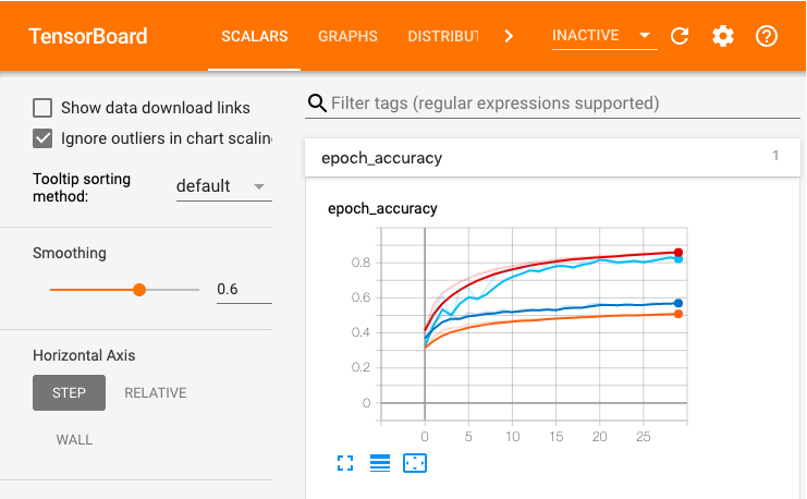
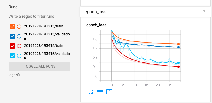
Below we can see the epoch accuracy and the epoch loss for train and testing data for both of the models.
In red we see the training performance for the minigooglenet, and in light blue the validation performance.
In orange we see the training performance for the shallownet and in normal blue the validation performance. Note that the model performs better on the validation data than on the training data, so it is likely that this model is underfit and we could increase the complexity. Of course the minigooglenet is in fact more complex and does in fact perform better.
%tensorboard --logdir logs/fit

