Implementing Ordinary Least Squares Linear Regression
Linear regression is an approach to modeling where the prediction is a linear combination of some model parameters and the input variables. In this notebook I implement two algorithms for linear regression: Simple Linear Regression and a Gradient Descent Algorithm for Ordinary Least Squares.
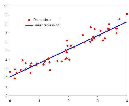
A popular way of generating (or estimating) the linear regression model is the Least Squares method. This method trains a model by finding the model that best reduces the square of the error between our training data and what our model would predict for the input variables of the training data.
It is possible to weight the errors when we apply this method. If we do not apply weights to the errors then we have what is called Ordinary Least Square. If we use Ordinary Least Square to calculate error then there is a closed form solution for finding the optimal parameters for a linear model used to predict the training data. Calculating this closed form solution is often itself called the Ordinary Least Squares “method” for solving the Linear Regression problem:
When there are only two dimensions (one independent, one dependent) then the Ordinary Least Squares method reduces to:
m = covariance(x, y) / variance (x)
c = mean(y) - m * mean(x)
This two dimensional variant of the closed form calculation of Ordinary Least Squares is called Simple Linear Regression.
When the close form solution of this problem is too computationaly expensive then we can use a gradient descent algorithm to solve for the parameters that minimizes the Ordinary Least Squares error.
Reference for Dataset: Swedish Committee on Analysis of Risk Premium in Motor Insurance
Thanks to machinelearningmaster.com and oreilly online learning for educational resources
Simple Linear Regression
Following https://machinelearningmastery.com/implement-simple-linear-regression-scratch-python/ I implement simple linear regression.
# Import Libraries
from random import seed
from random import randrange
from csv import reader
from math import sqrt

from matplotlib import pyplot as plt
%matplotlib inline
# Import Data
dataset = list()
with open('swedishinsurance.csv', 'r', encoding='utf-8-sig') as file:
    csv_reader = reader(file)
    for row in csv_reader:
        if not row:
            continue
        row = (float(row[0]), float(row[1]))
        dataset.append(row)
# Check dataset
dataset[:5]
[(108.0, 392.5), (19.0, 46.2), (13.0, 15.7), (124.0, 422.2), (40.0, 119.4)]
# Splitting dataset into training and testing data with test size being 40% of data
seed(1)
test = []
test_size = .33 * len(dataset)
train = list(dataset)
while len(test) < test_size:
    rand_index = randrange(len(train))
    test.append(train.pop(rand_index))
print(len(dataset), len(train), len(test))
63 42 21
#splitting train and test data into input and target vectors
x_train = [row[0] for row in train]
y_train = [row[1] for row in train]

x_test = [row[0] for row in test]
y_test = [row[1] for row in test]
def mean(values):
    return sum(values) / float(len(values))
def variance(values, mean):
    return sum([(x-mean)**2 for x in values])
def covariance(x, mean_x, y, mean_y):
    covar = 0.0
    for i in range(len(x)):
        covar += (x[i] - mean_x) * (y[i] - mean_y)
    return covar
# Using covariance and variance to estimate a linear 2 dimensional model

# Calculating mean of x and y, variance of x and covariance of x, y
mean_x, mean_y = mean(x_train), mean(y_train)
var_x = variance(x_train, mean_x)
covar_xy = covariance(x_train, mean_x, y_train, mean_y)

# Calculating parameters of 2-d linear regression model
m = covar_xy/var_x
c = mean(y_train) - m * (mean_x)

print(f'm = {m:.2f}, c={c:.2f}')
m = 3.39, c=16.57
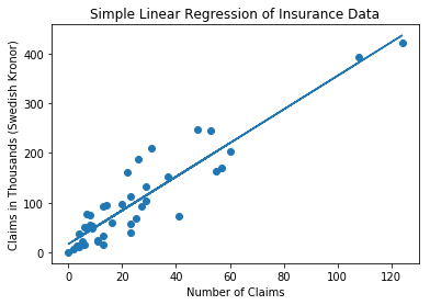
# plotting scatter plot of training data and graph
plt.scatter(x_train, y_train)
plt.plot(x_train, [m * x + c for x in x_train])
plt.xlabel('Number of Claims')
plt.ylabel('Claims in Thousands (Swedish Kronor)')
plt.title('Simple Linear Regression of Insurance Data')
plt.show()
# make predictions on test data
predictions = [m*x+c for x in x_test]
# evaluating predictions using root mean squared error
def calc_rmse(actuals, predictions):
    sum_square_errors = 0.0
    for i in range(len(predictions)):
        prediction_error = predictions[i] - actuals[i]
        sum_square_errors += prediction_error**2
    mse = sum_square_errors / float(len(predictions))
    return sqrt(mse)
rmse = calc_rmse(y_test, predictions)
print(f'RMSE: {rmse:.3f} thousands of Kronor')
RMSE: 33.711 thousands of Kronor
Estimating Ordinary Least Squares Model using Gradient Descent Method
Following https://learning.oreilly.com/library/view/python-machine-learning/9781783555130/ch10s03.html
This implementation uses linear algebra and applies to inputs with multiple variables. Often Gradient Descent is applied using partial derivatives, in this case we just use the error and the learning rate.
import numpy as np
from collections import defaultdict
# requires that X has a 1 all down its first column
# This algorithm is very sensitive to the learning rate
# Attempted to account for this by scaling it with the max of the y values

class LinearRegressionSGD(object):

    def __init__(self, standard_eta=0.01, n_iter=20):
        self.stdeta = standard_eta
        self.n_iter = n_iter

    def fit(self, X_train, y_train):
        self.coef_ = np.zeros(X_train.shape[1])
        self.iterations_ = defaultdict(dict)

        for i in range(self.n_iter):
            predicted = self.predict(X_train)
            errors = (predicted - y_train)
            self.iterations_[i]['coef'] = (self.coef_[0], self.coef_[1])
            delta_coef = -self.stdeta/max(y_train) * X_train.T.dot(errors)
            self.coef_ += delta_coef
            cost = (errors**2).sum()
            self.iterations_[i]['cost'] = cost
        return self

    def fitted_model(self):
        return self.iterations_[self.n_iter-1]

    def predict(self, X):
        return np.dot(X, self.coef_)
X_train = np.asarray([[1, x] for x in x_train])
X_test = np.asarray([[1, x] for x in x_test])
X_train.shape
(42, 2)
lr = LinearRegressionSGD()
lr.n_iter=10
lr.fit(X_train, y_train)
lr.fitted_model()
{'coef': (0.1489187247362218, 3.706856496264331), 'cost': 61899.13426903996}
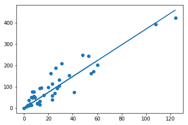
plt.scatter([x[1] for x in X_train], y_train)
plt.plot([x[1] for x in X_train], lr.predict(X_train))
[<matplotlib.lines.Line2D at 0x1206ff4a8>]
# make predictions on test data
predictions = lr.predict(X_test)
# evaluating predictions using root mean squared error
def calc_rmse(actuals, predictions):
    sum_square_errors = 0.0
    for i in range(len(predictions)):
        prediction_error = predictions[i] - actuals[i]
        sum_square_errors += prediction_error**2
    mse = sum_square_errors / float(len(predictions))
    return sqrt(mse)
rmse = calc_rmse(y_test, predictions)
print(f'RMSE: {rmse:.3f} thousands of Kronor')
RMSE: 38.181 thousands of Kronor
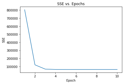
# plotting the decrease in our cost function over iterations
def plot_cost_v_epochs(lr):
    plt.plot(range(1, lr.n_iter+1), [data['cost'] for epoch, data in lr.iterations_.items()])
    plt.ylabel('SSE')
    plt.xlabel('Epoch')
    plt.title('SSE vs. Epochs')
    plt.show
def plot_2d_iterations(lr, X, y):
    n_iter = lr.n_iter
    step_size = int(n_iter/3)
    steps = [n_iter-i*step_size-1 for i in range(3)]
    steps.extend([2,1,0])
    steps.reverse()
    for i in steps:
        c = lr.iterations_[i]['coef'][0]
        m = lr.iterations_[i]['coef'][1]
        cost = lr.iterations_[i]['cost']
        plt.scatter([x[1] for x in X], y)
        plt.plot([x[1] for x in X], [m*x[1]+c for x in X])
        plt.xlabel('x')
        plt.ylabel('y')
        plt.title(f'Graph for {i+1} iteration, SSE: {cost:.1f}')
        plt.show()
plot_cost_v_epochs(lr)
plot_2d_iterations(lr, X_train, y_train)
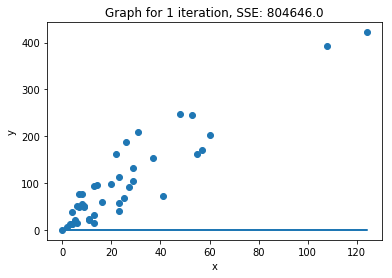
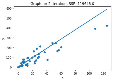
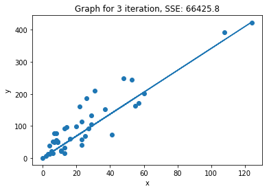

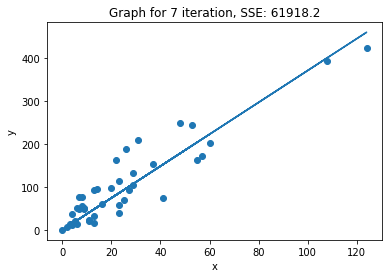

We can see that within 3 iterations we have almost reached the minimum of the cost function.
# Experimenting with Stochastic Gradient Descent on toy dataset
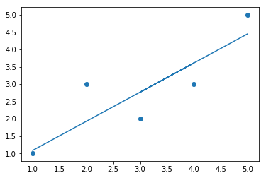
toy_data = dataset = [[1, 1], [2, 3], [4, 3], [3, 2], [5, 5]]
toy_x = [row[0] for row in dataset]
toy_y = [row[1] for row in dataset]
toy_X = np.asarray([(1, x) for x in toy_x])
lr = LinearRegressionSGD()
lr.fit(toy_X, toy_y)
lr.fitted_model()
{'cost': 2.4213693720663207, 'coef': array([0.24730859, 0.84061339])}
plt.scatter(toy_x, toy_y)
plt.plot(toy_x, lr.predict(toy_X))
[<matplotlib.lines.Line2D at 0x1200f0780>]
